Nonidentifiable models
[2]:
import warnings

import numpy as np
import polars as pl
import numba
import scipy.optimize
import scipy.stats as st

import iqplot

import bebi103

import bokeh.io
import bokeh.plotting
bokeh.io.output_notebook()
In this portion of the lesson, we will show how nonidentifiability can be lurking in an analysis.
The theoretical model
A human immunodeficiency virus (HIV) is a virus that causes host organisms to develop a weaker, and sometimes ineffective, immune system. HIV inserts its viral RNA into a target cell of the immune system. This virus gets reverse transcribed into DNA and integrated into the host cell’s chromosomes. The host cell will then transcribe the integrated DNA into mRNA for the production of viral proteins and produce new HIV. Newly created viruses then exit the cell by budding off from the host. HIV carries the danger of ongoing replication and cell infection without termination or immunological control. Because CD4 T cells, which communicate with other immune cells to activate responses to foreign pathogens, are the targets for viral infection and production, their infection leads to reductions in healthy CD4 T cell production, causing the immune system to weaken. This reduction in the immune response becomes particularly concerning after remaining infected for longer periods of time, leading to acquired immune deficiency syndrome (AIDS).
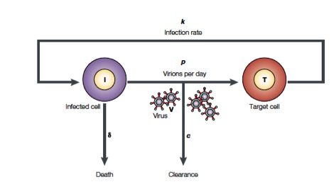
Perelson and coworkers have developed mathematical models to study HIV populations in the eukaryotic organisms. HIV-1 infects cells at a rate \(k\) and is produced from these infected T cells at a rate \(p\). On the other hand, the viruses are lost due to clearance by the immune system of drugs, which occurs at a rate \(c\), and infected cells die at a rate \(\delta\) (Figure from Perelson, Nat. Rev. Immunol., 2, 28-36, 2002)
The above process can be written down as a system of differential equations.
\begin{align} \frac{dT^*}{dt} &= k V_I T - \delta T^*\\[1em] \frac{dV_I}{dt} &= -cV_I\\[1em] \frac{dV_{NI}}{dt} &= N \delta T^{*} - c V_{NI}, \end{align}
Here, \(T(t)\) is the number of uninfected T-cells at time \(t\), and \(T^*\) is the number of infected T cells. Furthermore, there is a concentration \(V_I(t)\) of infectious viruses that infect T cells at the rate \(k\). We also have a concentration \(V_{NI}\) of innocuous viruses. We define \(N(t)\) to be the number of newly produced viruses from one infected cell over this cell’s lifetime. We can measure the total viral load, \(V(t) = V_I(t) + V_{NI}(t)\). If we initially have a viral load of \(V(0) = V_0\), we can solve the system of differential equations to give
\begin{align} V(t;V_0,c,\delta) = V_0e^{-ct} + \frac{cV_0}{c-\delta}\left[\frac{c}{c-\delta}(e^{-{\delta}t} - e^{-ct}) - {\delta}te^{-ct}\right]. \end{align}
The data set
We will take viral load data from a real patient (which you can download here). The patient was treated with the drug Ritonavir, a protease inhibitor that serves to clear the viruses; i.e., it modulates \(c\). So, in the context of the model, \(c\) is a good parameter to use to understand the efficacy of a drug.
Let us take a quick look at the data set.
[3]:
df = pl.read_csv(os.path.join(data_path, "hiv_data.csv"), comment_prefix="#")

p = bokeh.plotting.figure(
    frame_height=250,
    frame_width=450,
    x_axis_label="days after drug administration",
    y_axis_label="RNA copies per mL",
)
p.scatter(df["Days after administration"], df["RNA copies per mL"])

bokeh.io.show(p)
After some noisy viral RNA levels early on, the virus begins to be cleared after about a day, bringing the viral load down.
The statistical model
For our statistical model (which we will later see is nonidentifiable), we will assume that residual \(i\) is Normally distributed with scale parameter \(\sigma_i = \sigma_0 V(t_i;V_0, v, \delta)\). That is, we assume that the variability scales with the size of the measurement.
\begin{align} &\mu_i = V(t_i;V_0,c,\delta) = V_0e^{-ct_i} + \frac{cV_0}{c-\delta}\left[\frac{c}{c-\delta}(e^{-{\delta}t_i} - e^{-ct_i}) - {\delta}t_ie^{-ct_i}\right] \;\forall i, \\[1em] &V_i \sim \text{Norm}(\mu_i, \sigma_0 \mu_i) \;\forall i. \end{align}
Performing a regression to determine the parameters δ and c
The most common procedure to characterize the parameters δ and c is to minimize the sum of the square of the residuals between the theoretical equation given above and the measured data. As we showed in one of the homeworks, this is equivalent to finding the MAP parameter values for a model with a homoscedastic Gaussian likelihood and Uniform priors. Let’s proceed to do this MAP calculation.
In the viral load model, we need to make sure that we don’t get a divide by zero error when \(c \approx \delta\). We will use the fact that
\begin{align} \lim_{c\to\delta} V(t;V_0,c,\delta) = V_0 \left(1 + \delta t + \frac{\delta^2 t^2}{2}\right)\mathrm{e}^{-\delta t}. \end{align}
We can now write our viral load model. Because we will be computing the posterior on a grid for plotting later, I am going to use Numba to speed things up.
[4]:
@numba.njit
def viral_load_model(V0, c, delta, t):
    """Perelman model for viral load"""
    # If c and d are close, use limiting expression
    if abs(c - delta) < 1e-9:
        return V0 * (1 + delta * t + (delta * t) ** 2 / 2) * np.exp(-delta * t)

    # Proceed with typical calculation
    bracket_term = c / (c - delta) * (
        np.exp(-delta * t) - np.exp(-c * t)
    ) - delta * t * np.exp(-c * t)

    return V0 * (np.exp(-c * t) + c / (c - delta) * bracket_term)
I will now code up the statistical model. I will not use scipy.stats, opting for hand-coding the Normal log PDF by hand for speed.
[5]:
@numba.njit
def log_like_no_bounds(V0, c, delta, sigma_0, t, V):
    V_theor = viral_load_model(V0, c, delta, t)
    sigma = sigma_0 * V_theor

    return -np.sum(np.log(sigma)) - np.sum((V - V_theor)**2 / sigma**2) / 2


def log_likelihood(params, t, V):
    """Log likelihood for viral load model Gaussian."""
    if (params < 0).any():
        return -np.inf

    V0, c, delta, sigma_0 = params
    return log_like_no_bounds(V0, c, delta, sigma_0, t, V)
Based on the plot of the data, we will guess \(V_0 \approx 150000\) RNA copies/mL. We’ll guess that \(c\) is dominating the drop in load and choose \(c \approx 3\) days\(^{-1}\). We’ll guess \(\delta\) is slower, say 0.3 day\(^{-1}\). Now, we’ll perform the curve fit.
[6]:
# Unpack Numpy arrays for speed
t = df['Days after administration'].to_numpy()
V = df['RNA copies per mL'].to_numpy()

def mle(data):
    """Compute MLE for HIV model."""
    # Unpack
    t = data[:, 0]
    V = data[:, 1]

    # Initial guess
    p0 = np.array([150000, 3, 0.3, 0.3])

    # Find MLE
    with warnings.catch_warnings():
        warnings.simplefilter("ignore")
        res = scipy.optimize.minimize(
            fun=lambda p, t, V: -log_likelihood(p, t, V),
            x0=p0,
            args=(t, V),
            method='powell'
        )

    if res.success:
        return res.x
    else:
        raise RuntimeError('Convergence failed with message', res.message)

popt = mle(df[['Days after administration', 'RNA copies per mL']].to_numpy())

# Print results to screen
print("""MLEs:
V_0 = {0:.2e} copies of RNA/mL
  c = {1:.2f} 1/days
  δ = {2:.2f} 1/days
 σ0 = {3:.2f}
""".format(*popt))
MLEs:
V_0 = 1.32e+05 copies of RNA/mL
  c = 4.69 1/days
  δ = 0.44 1/days
 σ0 = 0.21
Now, we’ll plot the regression line with the data. This is what is commonly done, and indeed was done in the Perelson paper, though we will momentarily do a graphical model check, which is a better way to construct the plot.
[7]:
# Plot the regression line
t_smooth = np.linspace(0, 8, 200)
p.line(t_smooth, viral_load_model(*popt[:-1], t_smooth), color="orange", line_width=2)

bokeh.io.show(p)
Graphical model check
We’ll now perform a quick graphical model check, using our generative model parametrized by the MLE to generate data sets. First, we’ll code up a function to generate samples and then generate them.
[8]:
rng = np.random.default_rng()

def sample_hiv(V0, c, delta, sigma_0, t, size=1, rng=rng):
    """Generate samples of of HIV viral load curves"""
    samples = np.empty((size, len(t)))

    for i in range(size):
        mu = viral_load_model(V0, c, delta, t)
        samples[i] = np.maximum(0, rng.normal(mu, sigma_0*mu))

    return samples

t_theor = np.linspace(0, 8, 200)
samples = sample_hiv(*popt, t_theor, size=10000)
And now we can build the plot.
[9]:
p = bebi103.viz.predictive_regression(
    samples=samples,
    samples_x=t_theor,
    data=df[['Days after administration', 'RNA copies per mL']].to_numpy(),
    x_axis_label='days after drug administraion',
    y_axis_label='RNA copies per mL',
)

bokeh.io.show(p)
This looks ok, with most measured points falling within the middle 95th percentile of the generated data sets.
Confidence intervals of parameters
We can proceed to compute confidence intervals for the parameters. We will use our usual method of parametrically drawing new data sets out of the generative distribution parametrized by the MLE. WE first have to write a function to generate new data sets out of the model with the requisite call signature for bebi103.bootstrap.draw_bs_reps_mle().
[10]:
def gen_hiv(params, t, size, rng):
    return np.vstack((t, sample_hiv(*params, t, size=len(t), rng=rng))).transpose()

bs_reps = bebi103.bootstrap.draw_bs_reps_mle(
    mle,
    gen_hiv,
    data=df[["Days after administration", "RNA copies per mL"]].to_numpy(),
    mle_args=(),
    gen_args=(t,),
    size=10000,
    n_jobs=3,
    progress_bar=True,
)

# Compute confidence intervals and take a look
pl.DataFrame(
    data=np.percentile(bs_reps, [2.5, 97.5], axis=0),
    schema=["V0*", "c*", "δ*", "σ0*"],
)
100%|████████████████████████████████████████████████████████████████████████████████| 3333/3333 [00:47<00:00, 70.26it/s]
100%|████████████████████████████████████████████████████████████████████████████████| 3333/3333 [00:47<00:00, 70.07it/s]
100%|████████████████████████████████████████████████████████████████████████████████| 3334/3334 [00:48<00:00, 69.16it/s]
/Users/bois/miniconda3/envs/bebi103_build/lib/python3.12/multiprocessing/resource_tracker.py:254: UserWarning: resource_tracker: There appear to be 1 leaked semaphore objects to clean up at shutdown
  warnings.warn('resource_tracker: There appear to be %d '
/Users/bois/miniconda3/envs/bebi103_build/lib/python3.12/multiprocessing/resource_tracker.py:254: UserWarning: resource_tracker: There appear to be 1 leaked semaphore objects to clean up at shutdown
  warnings.warn('resource_tracker: There appear to be %d '
/Users/bois/miniconda3/envs/bebi103_build/lib/python3.12/multiprocessing/resource_tracker.py:254: UserWarning: resource_tracker: There appear to be 1 leaked semaphore objects to clean up at shutdown
  warnings.warn('resource_tracker: There appear to be %d '
[10]:
| V0* | c* | δ* | σ0* |
|---|---|---|---|
| f64 | f64 | f64 | f64 |
| 110018.869871 | 1.589742 | 0.390113 | 0.114634 |
| 154904.258234 | 3.7484e12 | 0.541423 | 0.261705 |
All parameters look like they have reasonable confidence intervals for their MLE except for \(c^*\). There is something funky, here, with the end of the confidence interval being \(10^{12}\) days\(^{-1}\)! We can take a quick look at the ECDF of our samples of \(c^*\).
[11]:
df_res = pl.DataFrame(data=bs_reps, schema=['V0*', 'c*', 'δ*', 'σ0*'])

p = iqplot.ecdf(
    data=df_res,
    q='c*',
    x_axis_type='log',
    x_axis_label='c* (1/days)',
)

bokeh.io.show(p)
Most samples are below 10, but we see 20% of them are well above 10, some positively enormous. This could be a solver issue, or it could be a lurking nonidentifiability. Let’s investigate.
Plotting the log likelihood function
To diagnose the issue, we will look at the likelihood function. To start with, we will fix the values of \(V_0\), \(\delta\), and \(\sigma_0\) to their MLEs and plot the likelihood function as a function of \(c\).
[12]:
# c values for plotting
c = np.linspace(0.01, 40, 300)

log_like = np.array(
    [log_likelihood(np.array([popt[0], c_val, *popt[-2:]]), t, V) for c_val in c]
)
like = np.exp(log_like - max(log_like))

p = bokeh.plotting.figure(
    frame_height=250,
    frame_width=450,
    x_axis_label="c (1/days)",
    y_axis_label="likelihood",
)
p.line(c, like, line_width=2)


bokeh.io.show(p)
This looks ok, though that tail looks a little troublesome. Let’s plot the log likelihood to better resolve it.
[13]:
# c values for plotting
c = np.linspace(0.01, 100, 300)

log_like = np.array(
    [log_likelihood(np.array([popt[0], c_val, *popt[-2:]]), t, V) for c_val in c]
)

p = bokeh.plotting.figure(
    frame_height=250,
    frame_width=450,
    x_axis_label="c (1/days)",
    y_axis_label="log likelihood",
)
p.line(c, log_like, line_width=2)

bokeh.io.show(p)
The log likelihood asymptotes to a constant value of \(c\), with all other parameters held at their MLE values.
Let’s take another look, considering also \(\delta\), plotting the likelihood function in the \(c\)-\(\delta\) plane.
[14]:
# c and δ values for plotting
c = np.linspace(0.01, 100, 200)
delta = np.linspace(0.2, 0.8, 200)

# Compute log-likelihood for each value
log_like = np.empty((200, 200))
for j, c_val in enumerate(c):
    for i, delta_val in enumerate(delta):
        log_like[i, j] = log_likelihood(
            np.array([popt[0], c_val, delta_val, popt[-1]]), t, V
        )

like = np.exp(log_like - log_like.max())

# Display the image
bokeh.io.show(
    bebi103.image.imshow(
        like,
        x_range=[c.min(), c.max()],
        y_range=[delta.min(), delta.max()],
        x_axis_label="c",
        y_axis_label="δ",
        frame_width=300,
        frame_height=300,
        flip=False,
    )
)
There is the nonidentifiability! The faint tail at \(\delta \approx 0.4\) days\(^{-1}\) goes off to infinity. If we have \(\delta \approx 0.4\), then any value of \(c\) will give roughly the same likelihood. From our estimates, we expect \(\delta\) to lie somewhere near 0.4 days\(^{-1}\), so this nonidentifiability is something we can likely encounter. It tells us that we cannot actually know \(c\) for sure, that is unless we had an independent measurement for \(\delta\). We would have no way of knowing this if we just solved the least squares problem and reported our values.
Computing the predictive regression and the confidence interval of the MLEs is the minimum you should do with your model. Next term, we will discuss principled modeling techniques that will help protect you from these pathologies that are encountered a lot more than we know.
Computing environment
[15]:
%load_ext watermark
%watermark -v -p numpy,polars,scipy,numba,bokeh,iqplot,bebi103,jupyterlab
Python implementation: CPython
Python version       : 3.12.4
IPython version      : 8.25.0

numpy     : 1.26.4
polars    : 1.2.1
scipy     : 1.13.1
numba     : 0.60.0
bokeh     : 3.4.1
iqplot    : 0.3.7
bebi103   : 0.1.21
jupyterlab: 4.0.13