Visualizing distributions

Data set download

---

import numpy as np
import pandas as pd

import iqplot

import bokeh.io
bokeh.io.output_notebook()

Loading BokehJS ...

---

You can think of an experiment as sampling out of a probability distribution. To make this more concrete, imagine measuring the lengths of eggs laid by a given hen. Each egg will by of a different length than others, but all of the eggs will be about six centimeters long. The probability of getting an egg more than eight centimeters long is very small, whereas the probability of getting an egg between 5.5 and 6.5 centimeters is high. The generative probability distribution, the distribution from which experimental data are sampled, then, has high probability mass around six centimeters and low probability mass away from that. We cannot know the generative distribution. We can approximate it with generative models (which we will do in the latter part of the course).

Here, we will investigate how to make plots to investigate properies about the (unknown) generative distribution of a set of repeated measurements. We will use the iqplot to make the plots, but will withhold dwelling on its syntax until the next notebook of this lesson. Instead, we will make a given plot and then discuss how it helps us visualize the underlying generative probability distribution of a data set.

We will continue using the facial recognition data set. We will make the usual adjustments by adding an 'insomnia' column and also a 'sleeper' column that more meaningfully indicates where the subject is an insomniac or a normal sleeper (with the words “normal” or “insomniac” instead of True and False).

fname = os.path.join(data_path, "gfmt_sleep.csv")
df = pd.read_csv(fname, na_values="*")
df["insomnia"] = df["sci"] <= 16
df["sleeper"] = df["insomnia"].apply(lambda x: "insomniac" if x else "normal")
df["gender"] = df["gender"].apply(lambda x: "female" if x == "f" else "male")

# Take a look as a reminder
df.head()

	participant number	gender	age	correct hit percentage	correct reject percentage	percent correct	confidence when correct hit	confidence incorrect hit	confidence correct reject	confidence incorrect reject	confidence when correct	confidence when incorrect	sci	psqi	ess	insomnia	sleeper
0	8	female	39	65	80	72.5	91.0	90.0	93.0	83.5	93.0	90.0	9	13	2	True	insomniac
1	16	male	42	90	90	90.0	75.5	55.5	70.5	50.0	75.0	50.0	4	11	7	True	insomniac
2	18	female	31	90	95	92.5	89.5	90.0	86.0	81.0	89.0	88.0	10	9	3	True	insomniac
3	22	female	35	100	75	87.5	89.5	NaN	71.0	80.0	88.0	80.0	13	8	20	True	insomniac
4	27	female	74	60	65	62.5	68.5	49.0	61.0	49.0	65.0	49.0	13	9	12	True	insomniac

Box plots

We saw in the previous part of the lesson that bar graphs throw out most of the information present in a data set. They only give an approximation of the mean of the generative distribution and nothing else. We can instead report more information.

A box-and-whisker plot, also just called a box plot is a better option than a bar graph. Indeed, it was invented by John Tukey himself. Instead of condensing your measurements into one value (or two, if you include an error bar) like in a bar graph, you condense them into at least five. It is easier to describe a box plot if you have one to look at.

p = iqplot.box(
    df,
    "percent correct",
    cats=["gender", "sleeper"],
    box_kwargs=dict(fill_color="#1f77b4"),
)

bokeh.io.show(p)

The top of a box is the 75th percentile of the measured data. That means that 75 percent of the measurements were less than the top of the box. The bottom of the box is the 25th percentile. The line in the middle of the box is the 50th percentile, also called the median. Half of the measured quantities were less than the median, and half were above. The total height of the box encompasses the measurements between the 25th and 75th percentile, and is called the interquartile region, or IQR. The top whisker extends to the minimum of these two quantities: the largest measured data point and the 75th percentile plus 1.5 times the IQR. Similarly, the bottom whisker extends to the maximum of the smallest measured data point and the 25th percentile minus 1.5 times the IQR. Any data points not falling between the whiskers are then plotting individually, and are typically termed outliers. Note that “outlier” is just a name; it does not imply anything special we should consider in those data points.

So, box-and-whisker plots give much more information than a bar plot. They give a reasonable summary of how data are distributed by providing quantiles.

Not to draw our focus away from visualizing how a data set is distributed, going forward in this notebook, we will not split the data set by gender and sleep preference, but will instead look at the entire data set. Here is a box plot for that.

p = iqplot.box(df, "percent correct", frame_height=100)
p.yaxis.visible = False

bokeh.io.show(p)

Plot all your data

While the box plot is better than a bar graph because it shows quantiles and not just a mean, it is still hiding much of the structure of the data set. Conversely, when plotting x-y data in a scatter plot, you plot all of your data points. Shouldn’t the same be true for plots with categorical variables? You went through all the work to get the data; you should show them all!

Strip plots

One convenient way to plot all of your data is a strip plot. In a strip plot, every point is plotted.

p = iqplot.strip(df, "percent correct", frame_height=100)
p.yaxis.visible = False

bokeh.io.show(p)

An obvious problem with this plot is that the data points overlap. We can get around this issue by adding a jitter to the plot. Instead of lining all of the data points up exactly in line with the category, we randomly “jitter” the points about the centerline, of course maintaining their position along the quantitative axis.

p = iqplot.strip(df, "percent correct", frame_height=100, spread="jitter")
p.yaxis.visible = False

bokeh.io.show(p)

Alternatively, we can deterministically spread the points in a swarm plot, where the glyphs are positioned so as not to overlap, but retain the same position along the quantitative axis.

p = iqplot.strip(df, "percent correct", frame_height=100, spread="swarm")
p.yaxis.visible = False

bokeh.io.show(p)

This plot allows us to make out how the data are distributed. We suspect there is more probability density around 85% or so, with a heavy tail heading toward lower values, ending at 40.

Spike plots

The swarm plot above essentially provides a count of the number of times a given measurement was observed. Because of the nature of the GFMT, the percent correct values are discrete, coming in 2.5% increments. When we have discrete values like that, a spike plot serves to provide the counts of each measurement value.

p = iqplot.spike(df, "percent correct")

bokeh.io.show(p)

Each spike rises to the number of times a given value was measured.

Spike plots fail, however, when the measurements do not take on discrete values. To demonstrated, we will add random noise to the percent correct data and try replotting. (We will learn about random number generation with NumPy in a future lesson. For now, this is for purposes of discussing plotting options.)

# Add a bit of noise to the % correct meas. so they are no longer discrete
rg = np.random.default_rng()
df["percent correct with noise"] = df["percent correct"] + rg.normal(
    0, 0.5, size=len(df)
)

# Replot swarm plot
p = iqplot.strip(df, "percent correct with noise", frame_height=100, spread="swarm")
p.yaxis.visible = False

bokeh.io.show(p)

We can still roughly make out how the data are distributed in the swarm plot, but the spike plot adds little beyond what we would see with a strip plot sans swarm or jitter.

p = iqplot.spike(df, "percent correct with noise", frame_height=100)

bokeh.io.show(p)

Histograms

If we do not have discrete data, we can instead use a histogram. A histogram is constructed by dividing the measurement values into bins and then counting how many measurements fall into each bin. The bins are then displayed graphically.

A problem with histograms is that they require a choice of binning. Different choices of bins can lead to qualitatively different appearances of the plot. One choice of number of bins is the Freedman-Diaconis rule, which serves to minimize the integral of the squared difference between the (unknown) underlying probability density function and the histogram. This is the default of iqplot.

p = iqplot.histogram(df, "percent correct with noise")

bokeh.io.show(p)

The rug plot at the bottom of the histogram shows all of the measurements (following the “plot all your data” rule).

ECDFs

Histograms are typically used to display how data are distributed. As an example I will generate Normally distributed data and plot the histogram.

x = rg.normal(size=500)
bokeh.io.show(iqplot.histogram(x, rug=False, style="step_filled"))

This looks similar to the standard Normal curve we are used to seeing and is a useful comparison to a probability density function (PDF). However, Histograms suffer from binning bias. By binning the data, you are not plotting all of them. In general, if you can plot all of your data, you should. For that reason, I prefer not to use histograms for studying how data are distributed, but rather prefer to use ECDFs, which enable plotting of all data.

The ECDF evaluated at x for a set of measurements is defined as

\begin{align} \text{ECDF}(x) = \text{fraction of measurements } \le x. \end{align}

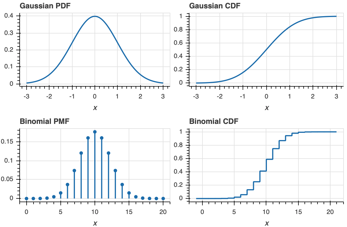
While the histogram is an attempt to visualize a probability density function (PDF) of a distribution, the ECDF visualizes the cumulative density function (CDF). The CDF, \(F(x)\), and PDF, \(f(x)\), both completely define a univariate distribution and are related by

\begin{align} f(x) = \frac{\mathrm{d}F}{\mathrm{d}x}. \end{align}

The definition of the ECDF is all that you need for interpretation. For a given value on the x-axis, the value of the ECDF is the fraction of observations that are less than or equal to that value. Once you get used to looking at CDFs, they will become as familiar as PDFs. A peak in a PDF corresponds to an inflection point in a CDF.

To make this more clear, let us look at plot of a PDF and ECDF for familiar distributions, the Gaussian and Binomial.

Now that we know what an ECDF is, we can plot it.

bokeh.io.show(iqplot.ecdf(x, style='dots'))

Each dot in the ECDF is a single data point that we measured. Given the above definition of the ECDF, it is defined for all real \(x\). So, formally, the ECDF is a continuous function (with discontinuous derivatives at each data point). So, it could be plotted like a staircase according to the formal definition.

bokeh.io.show(iqplot.ecdf(x, style="staircase"))

Either method of plotting is fine; there is not any less information in one than the other.

Let us now plot the percent correct data as an ECDF, both with dots and as a staircase. Visualizing it this way helps highlight the relationship between the dots and the staircase.

p = iqplot.ecdf(df, "percent correct")
p = iqplot.ecdf(df, "percent correct", p=p, style='dots', marker_kwargs=dict(color="orange"))

bokeh.io.show(p)

The circles are on the concave corners of the staircase.

Computing environment

%load_ext watermark
%watermark -v -p numpy,pandas,bokeh,iqplot,jupyterlab

Python implementation: CPython
Python version       : 3.11.5
IPython version      : 8.15.0

numpy     : 1.24.3
pandas    : 2.0.3
bokeh     : 3.2.1
iqplot    : 0.3.5
jupyterlab: 4.0.6