Homework 8.1: MLE for a ligand-gated ion channel (100 pts)
Caltech’s Henry Lester has been studying nicotinic acetylcholine receptors for decades. A schematic of the receptor, which is an ion channel, and its five (four unique) subunits, adapted from the book Physical Biology of the Cell 2, is shown below.
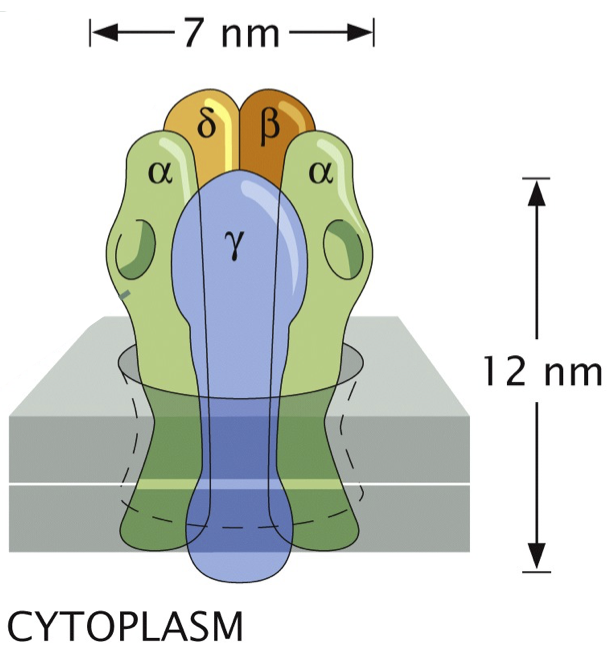
When acetylcholine ligands bind to the α units (the binding sites are shown as divots in the schematic), the channel opens and ions can flow through.
In a 1995 paper (Labarca, et al.), Labarca and coworkers in the Lester lab measured the (normalized) voltage across the ion channel for varying concentrations of acetylcholine. They did this for five different genotypes, shown below, where an asterisk denotes a mutation.
\(\alpha_2\beta\gamma\delta\) (wild type)
\(\alpha_2^*\beta\gamma\delta\)
\(\alpha_2\beta\gamma^*\delta\)
\(\alpha_2^*\beta\gamma^*\delta^*\)
\(\alpha_2\beta^*\gamma^*\delta^*\)
You can download the data set here.
We can work out theoretically that the fraction of time that an ion channel is open follows a logistic equation,
\begin{align} f_\mathrm{open}(c) = \frac{1}{1 + \mathrm{e}^{-\beta F(c)}}, \end{align}
where \(c\) is the concentration of acetylcholine, \(\beta = 1/k_B T\) is the inverse thermal energy, and \(F(c)\) is the Bohr parameter (named after Christian Bohr, the father of Nobel laureate Niels Bohr and of Danish national team footballer and mathematician Harald Bohr, and grandfather of Nobel laureate Aage Bohr), given by
\begin{align} F(c) = 2\Delta E_\mathrm{u} + 2 k_B T \ln\left(\frac{1+c/K_\mathrm{do}}{1+c/K_{dc}}\right). \end{align}
Here, \(\Delta E_\mathrm{u} = E_\mathrm{unbound}^\mathrm{closed} - E_\mathrm{unbound}^\mathrm{open}\) is the energy difference between the closed and open state of the ion channel without any acetylcholine bound, \(K_\mathrm{do}\) is the dissociation constant for acetylcholine binding the receptor when it is open, and \(K_\mathrm{dc}\) is the dissociation constant for acetylcholine binding the receptor when it is closed.
If we assume that in the limit of large concentrations the ion channel is completely open, then the normalized voltage \(v(c)\) across the channel is given by \(f_\mathrm{open}(c)\); \(v(c) = f_\mathrm{open}(c)\).
Before proceeding, I will note that I am structuring this problem such that you do what is typically done in many analyses I see in publications to expose how easy it is to make mistakes in statistical inference when working with models/data sets in which nonidentifiabilities lurk. We will visit this issue again in the last lecture of the term with another demonstration of how nonidentifiabilities can be problematic.
a) A common approach to parameter estimation is to find the so-called “best-fit” parameters and report them. “Best fit” is interpreted in a least squares sense and finding those parameters involves a least squares calculation in which the sum of the squares of the residuals is minimized. This approach is equivalent to performing a maximum likelihood estimate of a model in which the data are Normally distributed about the theoretical curve with a variance \(\sigma^2\) that is the same for all concentrations. Specifically,
\begin{align} v_i \mid c_i, \beta\Delta E_\mathrm{u}, K_\mathrm{do}, K_\mathrm{dc}, \sim \text{Norm}(v(c_i;\beta\Delta E_\mathrm{u}, K_\mathrm{do}, K_\mathrm{dc}), \sigma). \end{align}
For each of the five genotypes get the “best fit” parameters \(\beta\Delta E_\mathrm{u}\), \(K_\mathrm{do}\), \(K_\mathrm{dc}\). You do not need to compute confidence intervals for these estimates in this part, though you may in the next parts of the problem.
b) For each “best fit” parameter, plot the “best fit curve” along with the data. This is the theoretical curve parametrized by the parameters you found in part (a).
c) In my experience, the vast majority of analyses stop after part (b). TO GREAT PERIL! This model/data combination is an example of a case where quantitative interpretation of the estimates you get for the parameters would lead to erroneous conclusions. I will tell you now that this model is not identifiable with these measurements. (Remember, when we say a model is not identifiable, it means that we cannot unambiguously determine the parameter values. That is, two or more parameter sets are observationally equivalent.) You job in this part of the problem is to demonstrate that the model is not identifiable. You can use techniques we have learned in class to try to expose the nonidentifiabilities.